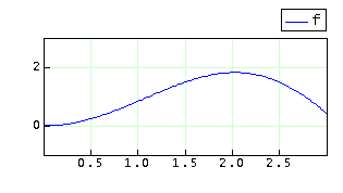
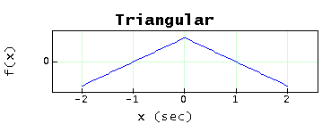
Figure 1. Plot of a function.
The syntax of the plot function is:
Where functionName is the name of the function to plot. Parameters x1 and x2 define the interval in which the function is going to be plotted. Parameter npts is the number of points used to make the plot. The program will divide the interval [x1,x2] into npts equally spaced points and find the value of the function at each point. The dots (...) stand for optional parameters controlling color, type (polar or Cartesian) and style.
Let's define a function to be used in the ongoing examples:
A plot of f is found as follows:
The program will open a window displaying the plot as shown in the Figure below.
The optional parameters may be a color, a style, a type, etc. The color may be "black", "blue", "cyan", "darkGray", "gray", "green", "lightGray", "magenta", "orange", "pink", "red", "white" or "yellow". The style may be "noline", "circle" or "square". The type may be "polar"; if no type is specified, the plot is assumed to be Cartesian.
In addition to the standard colors, you may enter a color with the same format used in HTML, e.g. "#aabbcc" where "aa" stands for the hexadecimal value of red, "bb" stands for the hexadecimal value of green and "cc" stands for the hexadecimal value of blue.
For instance, typing the line below creates the plot shown in Figure below.
By default, "circle" will fill a circle of size 4 pixels. To change the color to say green and the size to 12 pixels type:
If no fill is desired, type:
For a complete list of optional parameters, click the icon below.

The syntax to plot data stored in a matrix is the following:
Where M is the name of a matrix, xcol is the number of the column containing the "x" values, and ycol is the number of the column containing the "y" values. The dots stand for optional parameters to customize the plot.
For example:
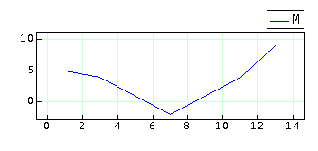
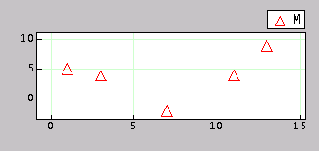
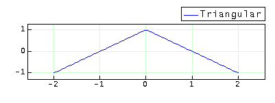
By default Calcugator joins each point with a blue line. To remove the line, place red triangular markers of size 12 pixels, and paint the canvas using light gray color, do:
Data stored in arrays can be plotted as follows:
where a and b are arrays storing (x,y) data. The dots stand for optional parameters. If no optional parameters are specified, then the Calcugator will draw filled circles in blue with a diameter of 4 pixels and no lines joining the points.
For example,
If you desire to use red circles of size 8 pixels and joint the points with green lines, do:
You may plot more than one function at the same time. Erase all previous plots (click the provided button) and type the following:
The resulting plot is shown below.
To plot parametric equations of the type,
build a vector function of type R-->R2,
and then use the plot function. The syntax to plot functions of type R-->R2 is equal to the one used to plot functions of type R-->R.
For example, given
a plot with a black color and a canvas color specified by #dddddd is obtained as follows,
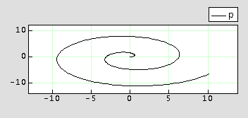
The optional parameters for selecting color and style apply similarly. Option "polar" is ignored for this type of plots.
Zooming, panning and selecting can be done using the mouse. To zoom, keep the Z key pressed and begin dragging the mouse. To pan, keep the P key pressed and begin dragging the mouse. To select, use the S key. The program has additional buttons to start zooming, panning and selecting.
To select the displayed region programmatically, use the optional parameter "window:xmin:xmax:ymin:ymax".
The intervals [xmin, xmax] and [ymin, ymax] define the region displayed in the plot.
For example:
Dragging the mouse begins tracing the plotted function. The trace displays the current value of x, f(x) and its derivative for the case of Cartesian plots.
For the case of polar plots, no derivative is drawn. Instead, the radius is displayed along with additional information.
The next plot illustrates the tracing of a polar plot in which no axes and no grid was selected.
By default, the name of the function is placed on the legend when you plot functions. If you plot matrix data, the name of the matrix is used instead. To customize the legend, use the option name:text. The text you enter will be put in the legend.
For example:
To remove the legend use the option "nolegend".
To place a title and custom labels on the axes, use options title:text and labels:xtext:ytext.
Option "swap" will swap the x and y axis of the plot. However, tracing information will be limited to the coordinates of points. No derivatives are reported.
For example:
Option "traceoff" will disable tracing information. This option is useful in client applications of the Calcugator graphics engine.
Other optional parameters include: "auto", "noauto", "stretch", "nostretch", "axes", "noaxes", "grid", "nogrid", "clear", or "dispose".
Option "auto" (default) stands for automatic finding of the window. The program finds the maximum and minimum values of the function in the plotting interval and adjusts the window so all values are shown. Option "noauto" restores the previous manual settings if any. When a plot is created a "window:-10:10:-10:10" is used by default.
Option "stretch" (default) stands for stretching the plot so to fit all available plotting space in the window. In most cases, this option results in non equal scales for the x and y axes. Using "nostretch" or unselecting the Stretch checkbox in the user interface would force the program to use equal scales when plotting. Figure below illustrates that case.
For a complete list of all optional parameters, click the link below.