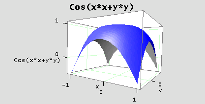
Figure 1. Example of a 3D plot.
Use function plot3D to create a surface plot as follows:
functionName is the name of the function to plot. functionName must be a function of type R2 to R (maps two-dimensional points into real numbers, e.g. f(x,y)=x*sin(y)).
Parameters x1, x2, y1 and y2 define the rectangular region in which the function is going to be evaluated. Parameters xnpts and ynpts are used as follows:
The interval [x1,x2] is divided into xnpts equally spaced points while the interval [y1,y2] is divided into ynpts equally spaced points defining a rectangular mesh. The function is evaluated at each mesh point.
The dots stand for optional parameters to customize the plot.
For example, the following lines:
create the plot shown in Figure 1 below.
For a complete list of optional parameters, click the icon below.

The user interface displaying the plot provides the following services:
You may choose the type of projection: Perspective (default) or Parallel.
You may rotate, translate or zoom the plot by pressing one of the following keys: R, P, C or Z, and at the same time, dragging the mouse.
R stands for rotation, P stands for translation, C stands for a rotation about a normal to the display, and Z stands for zooming.
In addition, keeping the key S pressed and dragging the mouse, you may select a region to zoom.
For example, rotating, translating and zooming the plot above, you may obtain the plot shown in Figure 2 below.
Additional buttons allow viewing the plot from standard points of view (default, top, front and right).
A list located to the bottom right, contains the names of the functions being plotted.
Two additional buttons allow you to delete the currently displayed plot or to dismiss the window.
Function plot3D has optional parameters. The general syntax is as follows:
The optional parameters may be one or many. To set a color you may type "black", "blue", "cyan", "darkGray", "gray", "green", "lightGray", "magenta", "orange", "pink", "red", "white", or "yellow".
Other colors can be specified using HTML format, e.g. "#aabbcc", where "aa" stands for the hexadecimal value of red, "bb" stands for the hexadecimal value of green, and "cc" stands for the hexadecimal value of blue.
To add a mesh on top of the surface, type "mesh".
For example, the plot in Figure 3 was built with the following line:
Sometimes a wireframe plot is more instructive. To plot using a wireframe style use "wireframe". For instance:
creates the plot shown below.
By default, the Calcugator graphics engine will scale the z axis in order that the plotted surface does not look too flat. If you need to scale the z axis, use the "scale:value" option, where "value" is a real number.
The example below will overwrite the default behavior of the graphics engine and the z values will be scaled by a factor of 2.5.
Function plot3D can create contour plots just by adding the optional parameter "contour". For example, the line below creates the plot in Figure 5.
Contour plots are best shown viewed from top and using a parallel projection. Clicking the Top button and selecting the option Parallel in the user interface, the plot above transforms to:
Function plot3D can also be used to create parametric plots. Given a function of type R to R3, e.g. f(t)=( cos(t), sin(t), t/10 ), a line plot can be created with the following syntax:
where functionName is the name of the function and t1 and t2 define the interval on which the function is to be evaluated. Calcugator will divide the interval [t1, t2] in npts equally spaced points and find the value of the function at those points.
The dots stand for optional parameters. For example, the following lines create the plot in Figure 7 below.
Mesh of points.
If you want to plot the z values corresponding to a rectangular mesh of points (x,y) like the one shown below:
                               x
  (1,  3,  1) (1,  3.5, .8) (1,  4,.95) (1,  4.5,1.1) (1,  5,1.3)
y (1.7,3, .8) (1.7,3.5, .9) (1.7,4,1.1) (1.7,4.5,1.3) (1.7,5,1.5)
  (3.1,3,1.1) (3.1,3,5,1.2) (3.1,4,1.5) (3.1,4.5,1.9) (3.1,5,1.5)
Enter the x and y values into two arrays and the z values into a matrix such that the rows of the matrix contain the y values for a given x. For the data shown above, the choice would be as follows:
To plot, use function plot3D:
Figure 8 below shows the resulting plot.
You may specify optional parameters like a color as described in section Optional parameters above.
By default a the plot is built using a mesh. To change the default select options "cube", "ball" or "bar". If "cube" is selected, the Calcugator draws a cube around each (x, y, z) point (top of the cube has the z coordinate). If "ball" is chosen, a sphere around the point is drawn. If "bar" is selected, a right prism with square section is drawn.
The next three plots are examples on using the optional parameters.
"cube" style.
"ball" style.
"cube" style and optional size.There are several optional parameters you may use to customize your plots. For example, the option "view:azimuth:elevation" allows you to programmatically rotate the plot.
Parameters azimuth and elevation define the angles used to rotate the plot. The azimuth is a rotation about a vertical axes. The elevation is a rotation about a line parallel to the horizon.
Other parameters may be "axes", "noaxes", "grid" or "nogrid", which may be used to turn on and off the drawing of the coordinate axes and background grid.
For example:
Moreover,
To place a title and custom labels on the axes, use options title:text and labels:xtext:ytext:ztext.
For example: