Statistical functions

Descriptive Statistics

All descriptive statistics functions operate on data stored in either arrays or matrices. If the data is stored in a matrix, the descriptive measure is computed for each column.

The set of implemented functions includes: mean(), median(), mode(), geometricMean(), harmonicMean(), rootMeanSquare(), quantile(), inverseQuantile(), range(), sum(), variance(), varianceMLE(), standarDeviation(), meanDeviation, moment(), skew(), kurtosis(), kstatistics(), zeroMean(), standarize(), kurtosisExcess(), trimmedMean(), covariance(), covarianceMLE(), correlation(), autocorrelation(), max(), min().

Additional functions exist to sample and compute frequencies and probabilities. The following lines show examples of using some of the functions above.

Let's store some data in an array and find the mean of the values:

The sample variance and standard deviation are:

The maximum likelihood estimate of the variance is calculated as follows:

Let's create some random data in a matrix using function randommatrix(). The first two parameters define the number of rows and columns while the next to define the bounds of the generated values. In this case, we generate integers between 1 and 10.

The kurtosis of each column is computed as follows:

All other statistical measures are found in a similar way. If the data is stored in a matrix, then the descriptive measure is computed for each column. See detailed description of each function in the Function Reference.

Plotting the Data

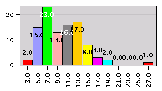
Depending on the nature of your data, several plotting options are available. Let's assume your data is stored in the array x below.

We use function frequencies() with a class width equal to 2.0. This function computes the number of data points withing each class. Function barchart() can be used to display the resulting matrix.

Figure 1. Displaying frequencies.

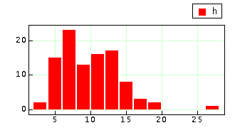
A custom plot can be prepared using function plot(). Function plot() can display the contents of any two columns of a matrix.

Figure 2. Custom plot. Class width equal to 2.0.

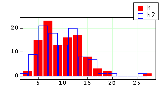
Let's select 1.0 as a new reference to create the classes, and compare the new plot.

Figure 3. Custom plot. Reference equal to 1.0.

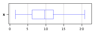
A box-and-whiskers plot of the data can be constructed as follows. Function boxwhiskers() expects the data stored in a matrix. Each row corresponds to a data set. In this case we build a matrix with one row only.

Figure 4. Box-and-whiskers plot of data.

Depending on your data, you may also use functions pie() or pareto().

Working the Data

There are several functions you may use to work your data, sort it, or find an arbitrary proportion.

Function sort() can be used to sort your data in ascending order.

Function apply() can modify each entry of an array or matrix. As an illustration, let's assume you need to square each entry and divide it by 3. You would start by defining a suitable function and applying it to each entry of the array as follows:

To find a proportion, use function findall(). For example, to find all the entries x such that 3<x<5, begin by defining a function and then use findall() as shown below. Function findall() would return an array with all the entries satisfying the condition.

Probability Distributions

Calcugator has a practical way of dealing with probability distributions; it treats a probability distribution like an "object" you create and you query for information.

To create a probability distribution use the distribution() function. For example, a StudentT distribution with 10 degrees of freedom is created as follows:

To find the value of the probability density function of this distribution at x=2.2, do:

To find the value of the cumulative probability for x=2.2, do:

To find the value of x such that the area of the left tail is 0.2, do:

To find the value of x such that the area of the right tail is 0.05, do:

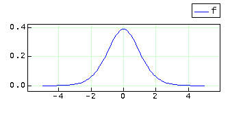
To create a plot of the distribution pdf, create a function and use the plot() function as follows:.

Figure 5. StudentT distribution (n=10.0).

A distribution object can also be used to generate random variates. For example, to generate 1000 random numbers from this distribution, do:

Notice the semicolon after the command. Using a semicolon cancels the display of the command's response. In this case we avoid displaying 1000 numbers.

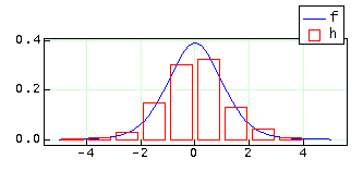
To see a visual display of the generated numbers, first use the probabilities() function. The first parameter is an array and the second is the class width. Using a class width equal to 1.0 we obtain the results below.

The first column of matrix h is the center of each class (bin) and the second column is the frequency of points in that class divided by the number of points. A histogram can be created by using the "bar" option in the plot() function. Notice that the plot() function can plot any two columns of a given matrix. In this case we plot column 1 versus column 2.

Figure 6. Random variates, StudentT (n=10.0)

The distribution object can also inform about the theoretical mean and variance.

Function pdfinfo() displays a summary of the probability function used by a distribution.

Supported Distributions

Here is a list of the supported distributions. Each one is presented with an example.

Poisson distribution

Geometric distribution

Logarithmic distribution

Binomial distribution

Negative binomial distribution

Hyper geometric distribution

Uniform discrete distribution

Chi square distribution

Non central Chi Square distribution

Non central Student-t distribution

Gaussian distribution

Gamma distribution

Uniform distribution

Beta distribution

Student-t distribution

Laplace distribution

Logistic distribution

Exponential distribution

F distribution

Non central F distribution

z-values

Functions snd() and invsnd() provide the so called z-values.

Standard Normal Distribution. Function snd(z) returns the area under the standard normal distribution from 0. to z (z>0). The function replaces the use of the typical tables found in textbooks.

Example:

Figure 7. Find area given z.

There is also a utility function invsnd(a) which returns the value z such that the area under the standard normal distribution curve is equal to a. Example:

Figure 8. Find z given area.

Random Values

The next group of functions are useful to generate sets of random results. Calcugator uses the Mersenne Twister algorithm as its core random engine.

• random() returns a random real number between 0. and 1.
• random(n) returns an array of size n with random numbers between 0. and 1.0.
• random(n,v) returns an array of size n with random values. If value v is real, all values are real between 0. and v. If value v is integer, all values are integers between 0 and v inclusive.
• random(n,v1,v2) returns an array of size n with random values. If any of the values v1 or v2 is real, all values are real between v1 and v2. If both values v1 and v2 are integer, all values integer between v1 and v2 inclusive.
• coin() returns either "H" (Heads) or "T" (Tails) at random.
• coin(n) returns an array of size n with random Heads and Tails.
• dice() returns a random integer between 1 and 6.
• dice(n) returns an array of size n with random integers between 1 and 6.
• die() returns two random integers between 1 an 6.
• die(n) returns an array of size n with random pairs of integers between 1 and 6.

Linear Regression

Use function linearreg to find the least squares regression line:

• linearreg( x, y )

f is any name you choose and x and y are the arrays containing the x and and y coordinates respectively.

For example,

a least squares regression line is obtained as follows,

now you may use function g like any other user defined function.

Let's plot the data. Let's use blue squares of size 8 pixels, no fills, and let's join the points using gray lines,

Let's plot the linear regression line on the interval [4,14] using 30 points to build the line and using color red:

Figure 9. Linear regression example.

Another statistical measure of the linear regression model is the correlation coefficient. To obtain it, use function corrcoeff(x,y).

• c=corrcoeff(x,y) returns the correlation coefficient corresponding to the data in arrays x and y.

Example:

General Linear Models

What follows is an example of finding fitting parameters for a second degree polynomial using the Least Squares method. Assume the data is a set of values (x,y) stored in a matrix. Column 1 stores the x values and column 2 stores the y values.

Figure 10. Raw points.

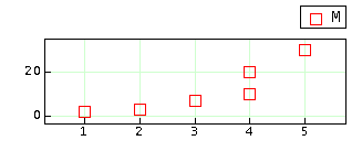
The x values and y values can be grabbed as follows:

Assuming the polynomial to fit is of the form y = b0 + b1*x + b2*x^2, the corresponding Vandermonde matrix is:

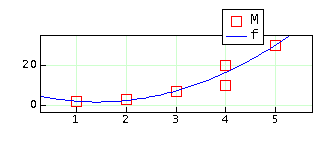
Finally, we solve for the parameters and build a function with them.

Figure 11. Fitted curve.

Principal Component Analysis

This section illustrates the use of some of the Linear Algebra functions in connection with statistical analysis. Given an observation matrix M where each row corresponds to an observation of a vector value, the covariance matrix can be found using the covariance() function.

The total variance is the trace of the covariance matrix.

The eigenvalues of S and the corresponding principal components (eigenvectors) are:

The transformed uncorrelated data can be computed as M*U.

Miscellaneous Functions

The following functions are implemented:

• sort(a) arranges all values stored in array a in increasing order.
• max(...) returns the maximum value of the arguments passed.
• min(...) returns the minimum value of the arguments passed.
• factorial(n) returns the factorial of integer n.
• combination(n,m) returns the number of combinations of m elements taken from a set of n elements.
• fibonacci(n) returns the n^th term of the Fibonacci series.
• sample(A,n) returns a sample of size n from array A.
• sample(A,n,m) returns a sample matrix with n rows and m columns. Each column is a sample of array A.
• probabilities(A,w) returns a matrix in which the first row are the middle point of classes with width w. The second column is the number of points in that class divided by the total number of points.
• probabilities(A,w,r). As above but the classes boundaries start at reference point r.
• frequencies(A,w)returns a matrix in which the first row are the middle point of classes with width w. The second column is the number of points in that class.
• frequencies(A,w,r). As above but the classes boundaries start at reference point r.